
Install fastdup
First, install fastdup and verify the installation.Roboflow Universe
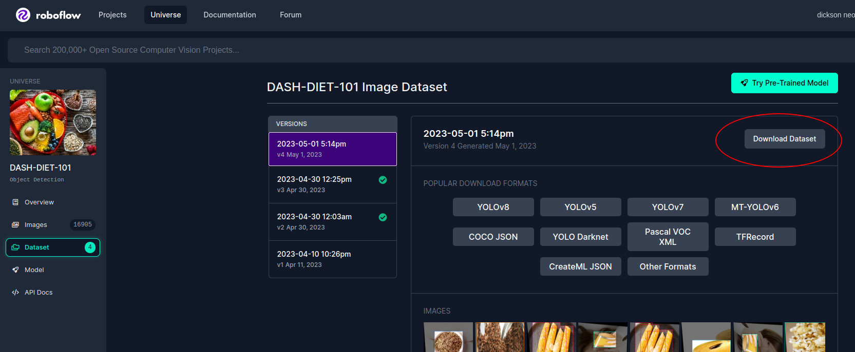
Roboflow Universe hosts over 200,000 computer vision datasets. In order to download datasets from Roboflow Universe, sign-up for free. Now, head over to https://universe.roboflow.com/ to search for the dataset of interest.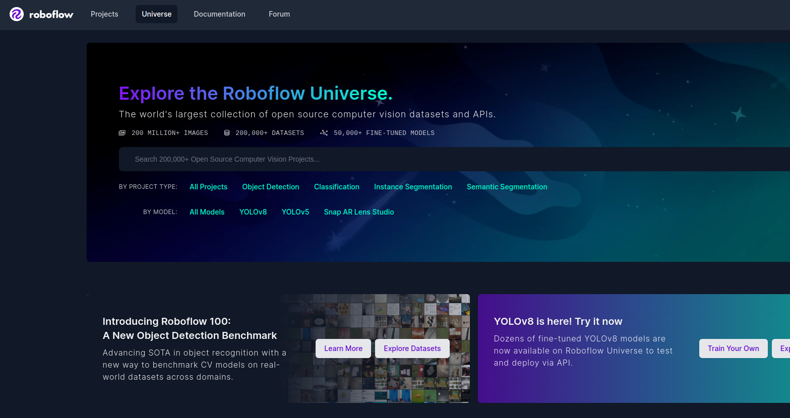 Once you find a dataset, click on the ‘Download Dataset’ button on the dataset page.
 A pop-up will appear with a code snippet to download the dataset into your local machine. Copy the code snippet.
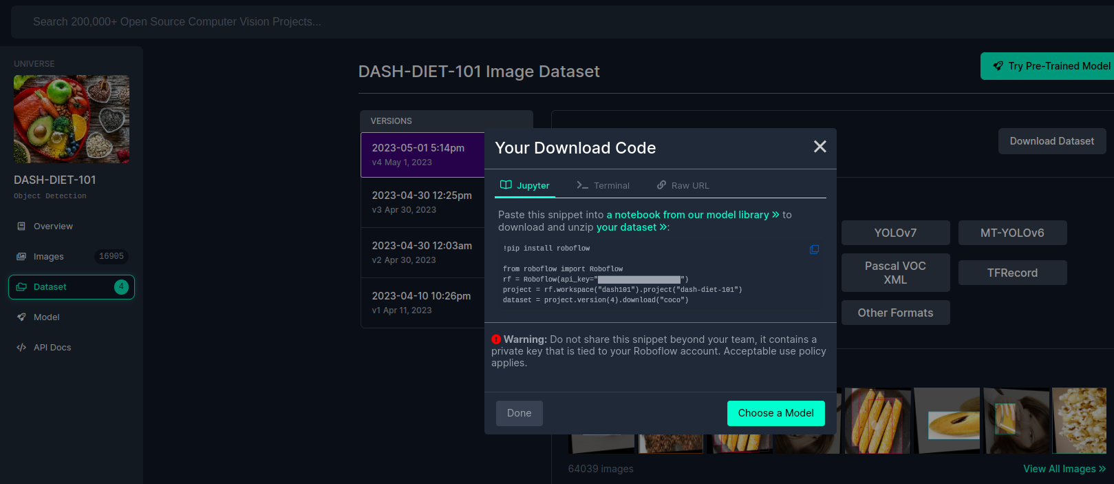
🚧 Warning The code snippet consists of an API key that is tied to your account. Keep it private.
Install Roboflow Python
The Roboflow Python Package is a Python wrapper around the core Roboflow web application and REST API. To install, run:
❗️ API Key
Replace YOUR_API_KEY with your own API key from Roboflow. Do not share this key beyond your team, it contains a private key that is tied to your Roboflow account.
Download Dataset
For this tutorial, let’s download the Dash Diet 101 Dataset in COCO annotations format into our local folder.DASH-DIET-101-4.
The DASH-DIET-101 dataset was created by Bhavya Bansal, Nikunj Bansal, Dhruv Sehgal, Yogita Gehani, and Ayush Rai with the goal of creating a model to detect food items that reduce Hypertension.
It contains 16,900 images of 101 popular food items with annotated bounding boxes.
Analyze Bounding Boxes with fastdup
To run fastdup, you only need to pointinput_dir to the folder containing images from the dataset.
run method.
Invalid Bounding Boxes
Since this dataset is annotated with bounding boxes, let’s check if all the bounding boxes are valid. Bounding boxes that are either too small or go beyond image boundaries are flagged as bad bounding boxes in fastdup. Let’s get the invalid bounding boxes.Label Distribution
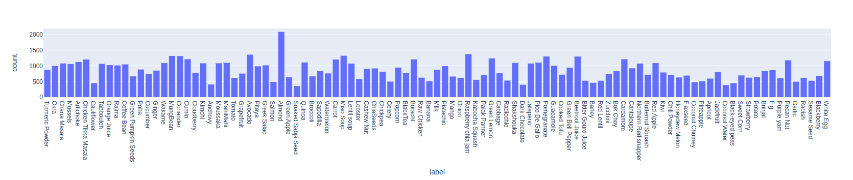
Let’s the label distribution in a bar chart.📘 Info This code snippet uses plotly to plot, install plotly with:
Bounding Box Size and Shape Issues
Objects come in various shapes and sizes, and sometimes objects might be incorrectly labeled or too small to be useful. We will now find the smallest, narrowest, and widest objects, and assess their usefulness. Let’s get the annotations and calculate the area and aspect ratio.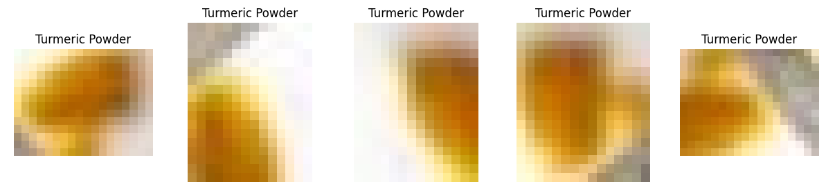 View the top and bottom-most extreme aspect ratio.

Visualize Issues with fastdup Gallery
There are several other methods we can use to inspect and visualize the issues found.Duplicates & Near-duplicates
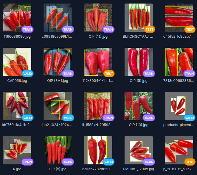
First, let’s visualize the duplicate images at the bounding box level.📘 Note The duplicates visualized here is at the bounding box level, NOT at the image level. In other words, the bounding box image is cropped from the original image and compared to other bounding box images for duplicates.
distance value of 1.0 indicates an exact duplicate.
As a sanity check, let’s show the images that are flagged as duplicates here.
Image Clusters
We can also view similar-looking images forming clusters.Bright/Dark/Blurry Images
We can show the brightest images from the dataset in a gallery. Changemetric to blur or dark to view blurry and dark images.
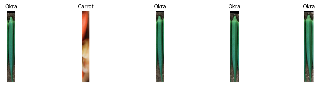
Mislabels
Wrap Up
That’s it! We’ve just conveniently surfaced many issues with this dataset by running fastdup. By taking care of dataset quality issues, we hope this will help you train better models. Questions about this tutorial? Reach out to us on our Slack channel!VL Profiler - A faster and easier way to diagnose and visualize dataset issues
The team behind fastdup also recently launched VL Profiler, a no-code cloud-based platform that lets you leverage fastdup in the browser. VL Profiler lets you find:- Duplicates/near-duplicates.
- Outliers.
- Mislabels.
- Non-useful images.
👍 Free Usage Use VL Profiler for free to analyze issues on your dataset with up to 1,000,000 images. Get started for free.Not convinced yet? Interact with a collection of dataset like ImageNet-21K, COCO, and DeepFashion here. No sign-ups needed.